Restaurant Demand Forecasting: How to Plan Covers
Learn restaurant demand forecasting step by step: data sources, methods, error metrics, and how to set staffing and seating from covers you can trust.

It's Friday at 18:40. The book shows 70 covers, the kitchen prepped for 70, and the rota matches 70. By 19:30, walk-ins are waiting at the door, two tables of six haven't shown, and the pass is backing up because 40 guests arrived in the same 20 minutes.
That night isn't a staffing failure. It's a forecasting failure. Restaurant demand forecasting that stops at a daily total can't tell you which party sizes to accept, when to pace arrivals, or which covers make money. Forecast accepted covers per shift and per party size, rank each pattern by contribution margin per seat hour, and the forecast starts driving seating, pacing, staffing and profit instead of just predicting a busy night.
Table of Contents
- Which Forecasting Method Fits Your Restaurant
- Data Sources to Pull Before You Start
- How to Build Your First Forecast in Five Steps
- Error Metrics That Show Whether Your Forecast Works
- Turning Covers Into Seating and Staffing Decisions
- Detect Demand Shifts Before They Break the Forecast
- Keep the Forecast Accurate Week to Week
Which Forecasting Method Fits Your Restaurant
You don't need machine learning on day one. The right method depends on how much clean history you have, not on how advanced a tool sounds.
Start with the seasonal naive baseline. Forecast this Friday as last Friday, this Tuesday as last Tuesday. It's crude, and that's the point. Every other method has to beat it on your own covers before it earns a place in your planning.
What Each Method Actually Costs You in Time
A spreadsheet model takes an afternoon to set up and an hour a week to maintain. A regression model needs calendar and weather data kept current. A gradient boosting model needs someone who can retrain it, check the features and explain why the number moved. If nobody in the building can do that on a Monday morning, the model won't survive its first bad week.
A restaurant-industry review of forecasting methods found that exponential-smoothing time-series models often performed as well as or better than econometric approaches while requiring less time and technical skill. For most independent restaurants, that's the sensible starting point. It weights recent weeks more heavily than old ones, handles weekday patterns, and runs in a spreadsheet.
| Method | Data needed | Effort | Best for |
|---|---|---|---|
| Seasonal naive (same weekday last week) | Last 8 weeks of daily covers | Very low | Baseline every other method must beat |
| Simple moving average | Last 4 to 8 weeks of daily covers | Very low | Steady lunch trade with little weekly variation |
| Exponential smoothing with weekday seasonality | 12 months of daily covers | Low | Most independent restaurants |
| Regression with weather, holidays and events | 1 to 2 years plus calendar and weather data | Medium | Venues with weather-sensitive terraces or event-driven nights |
| Gradient boosting (XGBoost) | 2 or more years with many features | High | Multi-location groups with clean reservation data |
The Rule for Choosing
Don't choose by ambition. Choose by proof.
Practical rule: Pick the simplest method that beats the seasonal naive baseline on the last eight weeks of covers, and keep it until a more complex method beats it by a margin worth the upkeep.
A moving average suits a steady weekday lunch where Tuesday rarely differs from Wednesday. It fails when terraces, school holidays or match nights drive the trade. That's when regression earns its keep, because you can add rain, temperature and events explicitly instead of hoping the average absorbs them.
Data Sources to Pull Before You Start
Start with what you already have. You don't need new software to pull the first dataset, you need consistent exports from systems you already run.
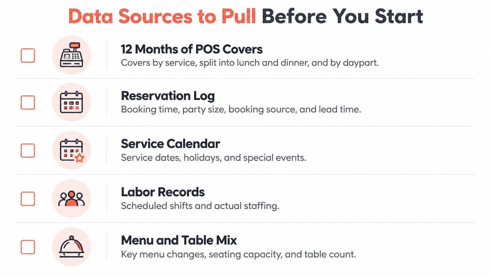
Pull at least 12 months of point-of-sale covers, split by location, service and daypart. Lunch and dinner behave differently, so never blend them. Add your reservation log with booking time, party size, booking channel, lead time and final status, meaning honored, cancelled or no-show. Add walk-in counts from the waitlist or door count, because refused walk-ins are demand too, just demand you didn't seat.
A recent restaurant forecasting study found the most influential inputs for predicting daily customer flow were the previous day's customer count, exponentially smoothed historical demand, holidays, day of the week, and weather, and its comparison found XGBoost had the lowest mean absolute error and mean squared error across all tested feature sets. You don't need that model to use the finding. It tells you which five inputs to collect first.
Outside Signals and Cleaning
Add historical weather for the same dates from a nearby station, public and school holiday calendars, local events such as matches, festivals and conferences, and your own promotion dates. A holiday Tuesday isn't a normal Tuesday, and your data should say so explicitly.
For Belgian operations, your GKS (Geregistreerd Kassasysteem) records give you a compliant, timestamped sales history to reconcile against covers. Use the GKS export as the check that POS covers and revenue line up by service, so a till error doesn't become a forecast error.
Then clean the history before you model anything:
- Closures flagged: Mark closure days, private buyouts and reduced-capacity nights, don't delete them.
- Sold-out nights separated: Flag services where you ran out of tables or key dishes, so capped sales aren't read as weak demand.
- No-shows split from cancellations: They have different causes and different fixes.
- Events logged: One line per event, with date and expected draw.
- Holiday weekdays tagged: Separate a holiday Tuesday from a normal Tuesday in the file itself.
How to Build Your First Forecast in Five Steps
This isn't a new idea dressed up in new software. A foodservice study published in 1992 using operational data from residence and dining-hall foodservices at Ohio State University forecast total customer counts with deseasonalized simple exponential smoothing, then estimated demand for individual menu items by multiplying the projected customer count by a predicted menu-preference statistic. All tested forecasting models were more accurate than the operations' existing methods, using a personal computer, spreadsheet and database software.
The logic still holds. First estimate how many guests arrive, then estimate how they split. In a dining room, that split means party size, arrival time and table configuration.
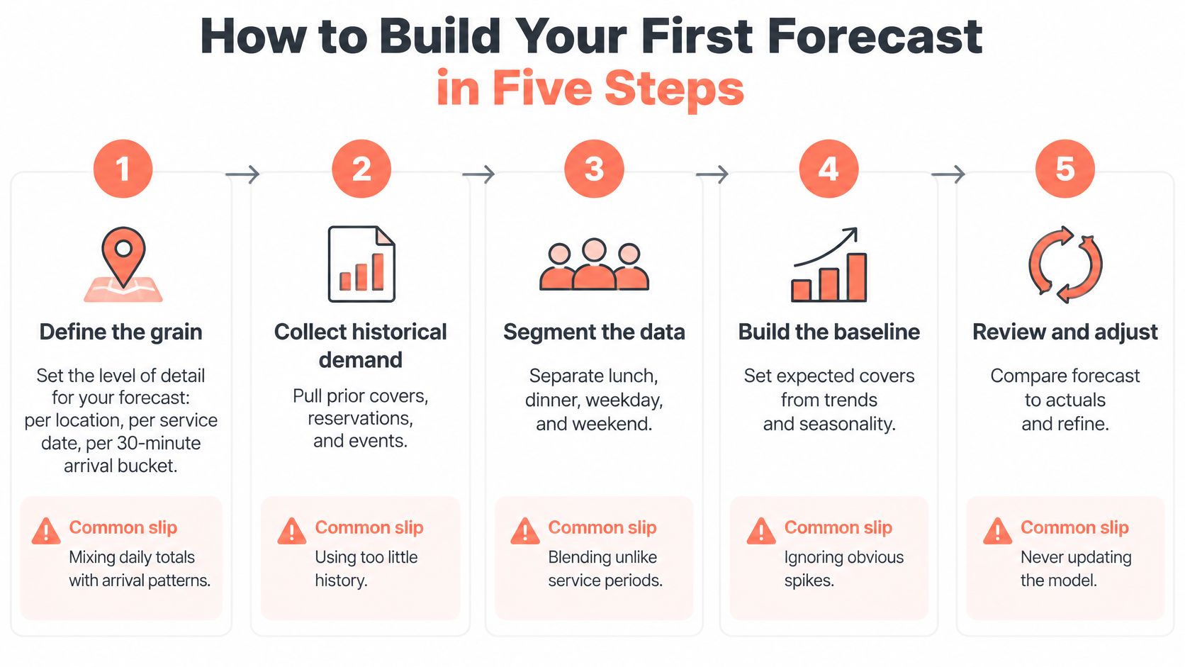
Step 1 Define the Grain
1. Define the grain before you touch a formula. Forecast covers per location, per service date, per 30-minute arrival bucket, separately for lunch and dinner. The forecast grain decides which decisions the number can support. A daily total can support ordering, but it can't support pacing.
Common slip: forecasting the whole day as one number, then discovering the rush all landed at 19:30.
Step 2 Build the Baseline
2. Build the baseline and compare it. Run exponential smoothing with weekday seasonality on the last 12 months, then run the seasonal naive forecast on the same period. Score both. If the smoothing model doesn't beat last week's same weekday, your data or your setup has a problem, and adding features will hide it rather than fix it.
Common slip: skipping the comparison, so there's no evidence the model adds anything over a guess.
Step 3 Add Adjustments From Your Own Nights
3. Add adjustments for holidays, rain and local events. Calculate each multiplier from your own past nights with the same condition. If rainy Saturdays ran lower on the terrace but held up inside, use two multipliers, not one. Keep a short log of the nights behind each multiplier so you can defend or retire it later.
Common slip: copying a holiday uplift from a different city or concept. A brasserie near a stadium and a fine dining room in a quiet street don't share event effects.
Step 4 Validate in Time Order
4. Validate on a rolling window. Train on the first nine months, test on the next month, roll forward and repeat. Time order matters because service never lets you peek at next month. This also shows whether accuracy holds across seasons or only in the months you happened to test.
Common slip: using a random train and test split, which lets future nights leak into training and flatters the result.
Step 5 Output a Range, Not a Number
5. Publish a central estimate with low and high bounds per bucket, plus one stress case, for example a rainy Saturday with a concert nearby. The range is what makes the forecast operational. It tells the host how much capacity to hold back and tells the GM when to call in the extra server.
A forecast bucket that doesn't map to a seating or staffing decision is reporting, not planning. If nobody changes anything when the number moves, drop the bucket or change the decision it feeds.
Common slip: planning prep, rota and table layout to the central number only, so any normal variation becomes a surprise.
Check the finished forecast bucket by bucket. Each 30-minute slot should answer three questions. How many covers, in what party sizes, and what does the room do differently at the low bound versus the high bound? If a bucket can't answer the third question, the work isn't finished yet.
Error Metrics That Show Whether Your Forecast Works
A single accuracy percentage misleads. A forecast can average out fine across a month and still miss every Friday, which is the night a miss costs you overtime, waste and refused walk-ins.
The 1992 Ohio State work made the same point in its own way, judging forecasts with several error metrics rather than one score. Customer-count errors and mix errors hit operations differently, so one number can't describe both. For a broader walkthrough of how these measures behave, PlotStudio AI's guide to forecasting accuracy is a useful companion when setting up your scoring sheet.
The Four Measures Worth Tracking
MAE is the easiest to explain in a kitchen. If MAE is 8 covers, the forecast misses by 8 covers on a typical service, and prep can be planned around that gap. RMSE answers a different question. It penalises large misses heavily, so it tells you how bad the bad nights get, the surprise peak that breaks the pass.
MAPE expresses the miss as a share of actual covers, which helps when comparing a 40-seat bistro with a 120-seat brasserie. It breaks down when a bucket sits near zero, such as Monday at 15:00, where a miss of two covers becomes a huge percentage. Bias shows direction. A forecast running low every Friday leaves you short exactly when you need staff most.
| Metric | What it measures | Use it when | Watch out for |
|---|---|---|---|
| MAE | Average miss in covers | Planning typical service volume | Treats a big miss and a small miss the same |
| RMSE | Size of large misses | Protecting against surprise peaks | Heavily affected by one outlier night |
| MAPE | Miss as a share of actual covers | Comparing venues of different sizes | Unstable when a bucket is near zero |
| Bias | Direction of errors over time | Spotting systematic over or under forecasting | Can hide offsetting misses |
Watch bias and MAE together. Positive and negative misses can offset, so bias can look near zero while MAE shows the forecast is missing badly in both directions. Setting this scoring up cleanly is part of basic restaurant data analytics, not a specialist project.
The Monday Routine
Score the last four weeks every Monday, by service and by bucket. Compare each measure against the seasonal naive baseline on the same weeks. A model that stops beating the baseline has stopped earning its upkeep.
Recalibrate when bias stays on one side for three weeks running. Before changing the method, check the inputs, because a run of misses usually traces back to an unlogged event, a changed opening pattern or sold-out nights polluting the history. Score only buckets that had real demand, so empty afternoon slots don't dilute the numbers that matter at service.
Turning Covers Into Seating and Staffing Decisions
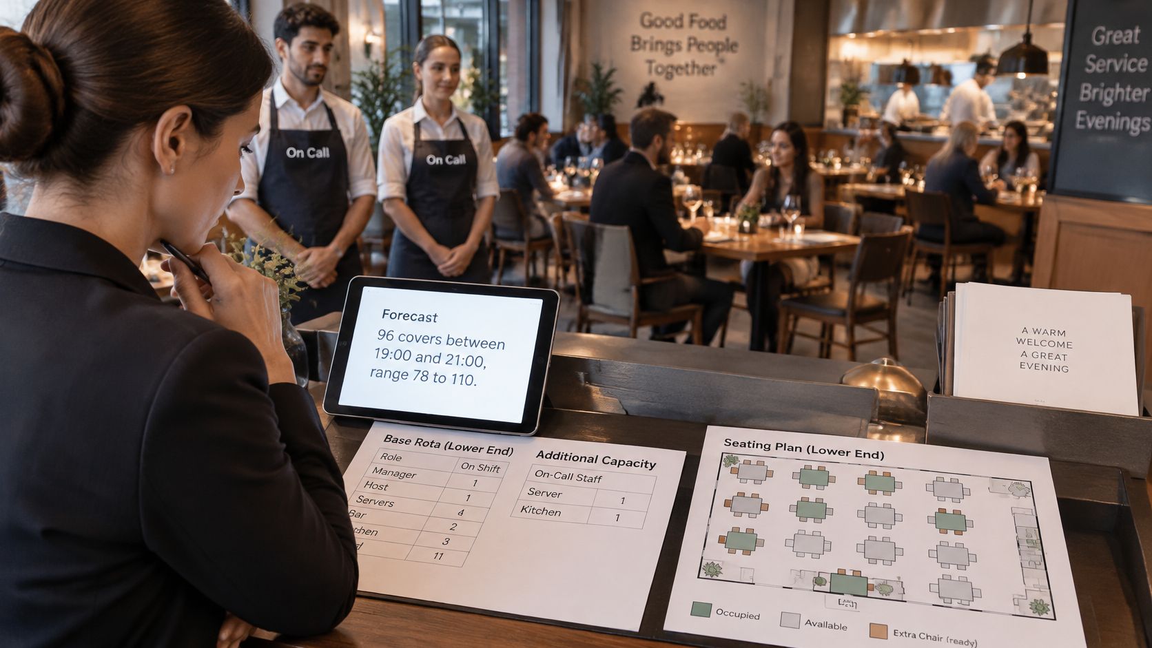
Say a Friday forecast gives 96 covers between 19:00 and 21:00, with a range of 78 to 110. That's a hypothetical worked example, but it's the shape a useful forecast takes. Plan the base rota and the initial table layout to the lower end, then release capacity as live bookings move toward the upper bound.
The manager reviewing the evening plan below is doing the conversion work, turning buckets into tables and sections before service starts.
Split the Forecast by Party Size
Ninety-six covers as tables of two is a completely different room from 96 covers as tables of four and six. Party size drives table configuration, service time and average spend. Forecast the mix from your reservation log by weekday and daypart, then set the floor accordingly, which is where a live restaurant seating chart earns its place during service rather than in the office.
Rank the patterns before the phone starts ringing. A four-top at 19:00 that turns by 21:00 usually beats a two-top that sits for three hours on the same table. When capacity tightens, accept in contribution order, not purely in booking order.
Correct for No-Shows With Your Own Rate
Bookings aren't covers. A 2024 OpenTable dataset cited in hospitality research reported that 28% of restaurant reservations made in the United States during the previous year were not honored. Treat that as context, not as your number. No-show rates vary by channel, cuisine, deposit policy and guest segment.
Measure your own rate by channel and by deposit status over the last 12 weeks. Overbook only by the margin that history supports, and only in the buckets where a spare table of the right size would free up. Overbooking a Friday peak on hope creates a queue, not covers.
The short video below shows how pacing arrivals against kitchen capacity looks in practice during a live service.
Pace Arrivals and Protect Walk-Ins
Set a pacing limit on arrivals per 15 minutes based on what the kitchen can fire without queues at the pass, not on how many chairs are empty. A forecast peak that ignores throughput just moves the bottleneck from the door to the kitchen.
Use the forecast spread to set walk-in allocation. When the range is wide, keep a larger share of tables unbooked, because uncertainty cuts both ways. When the range is narrow and bookings are tracking the central estimate, release more tables in advance.
Three decisions come out of this, and they shouldn't all change at once:
- Seating layout: Table sizes and joins set before service.
- Pacing rules: Maximum arrivals per 15 minutes, by service.
- Staffing levels: Base rota to the low bound, named on-call cover for the high bound.
Change pacing first. It's reversible mid-service, it protects ticket times immediately, and it tells you within one weekend whether the layout or the rota is the main constraint.
Detect Demand Shifts Before They Break the Forecast
A model only learns from history. When guest behaviour changes, a forecast built on last year's pattern doesn't get slightly worse, it misses in the same direction every week until someone intervenes.
Check four signals against your covers data each month:
- Spend per cover up, covers down: Guests may be spending more per head while ordering fewer items. Reporting on recent United States trading noted that United States restaurant spending was 23% above pre-pandemic levels while inflation-adjusted growth was only 0.8%. Separate nominal spend from real volume before calling it growth.
- Daypart migration: Dinner softening while lunch, early seatings or takeaway grow means the split you forecast separately is itself moving.
- Party-size mix shifting: More pairs and fewer sixes changes table demand even when total covers hold steady.
- Bias stuck on one side: Three weeks of misses in the same direction signals a regime change, not noise.
When a signal persists for three weeks, start a new baseline from the change date instead of averaging the old pattern with the new one. Averaging guarantees the forecast matches neither.
Tag one-off shocks, such as roadworks outside the door or a competitor closing for renovation, so they inform judgement without skewing the baseline.
Use the shift review to re-rank demand by contribution margin per seat hour. A table of two at 19:00 may earn less than a table of four at 21:00. When capacity is tight, the forecast should show which covers to accept first, which to pace later, and which to turn away politely.
Keep the Forecast Accurate Week to Week
Forecasts decay through neglect, not bad maths. A short weekly routine keeps the numbers honest and takes less time than rebuilding a rota mid-service.
The Weekly Routine
Every Monday, score last week's errors, update the log with closures, events and sold-out nights, then set expected covers for the next 14 days per 30-minute bucket. Fourteen days is far enough to order and roster, short enough that booking pace still corrects the estimate.
Then change three things and write down that you changed them. The rota for each service, the table layout, and the pacing rule for peak buckets. Good restaurant scheduling software makes the rota change fast, but the discipline of linking it to the bucket forecast is what saves labor cost.
Before touching the model, compare forecast against actuals line by line. Most error sits in the inputs, an unlogged buyout, a sold-out special, a channel promotion nobody told the GM about. Fix the log first.
| Mistake | Effect | Fix |
|---|---|---|
| Random train and test split | Model looks more accurate than it is | Use time-ordered rolling validation |
| Counting bookings as covers | Demand overstated by no-shows and cancellations | Track expected covers separately from bookings |
| Closures and private events left in history | Distorted baseline | Flag and exclude them |
| Single annual average | Misses weekday and seasonal patterns | Model by weekday and season |
| Whole day as one number | Misses when the rush actually hits | Forecast 30-minute arrival buckets |
| Sold-out nights recorded as weak demand | Demand underestimated | Log unmet demand as its own field |
What the Effort Pays Back
Treat published results as a benchmark to test against, not a promise. A peer-reviewed study of three foodservice operations using three to nine years of daily operating data found machine-learning forecasts could have reduced wasted meals by 14% to 52% and unmet demand by 3% to 16% compared with existing methods.
Run the arithmetic on your own write-offs. If you write off €500 of food a week, a 14% cut saves €70 a week, roughly €3,600 a year, before counting recovered sales from fewer sold-out dishes. Track waste value and sold-out nights for four weeks to measure your own result rather than borrowing someone else's.
The seating side compounds the saving. Restaurants using 10Seat see 30% more reservations, 40% fewer no-shows and 10-15% more covers per shift, and its smart scheduling engine includes predictive no-show detection, automatic table optimization, and dynamic pricing recommendations. Tools such as TheFork, OpenTable, Zenchef and Formitable typically charge per cover, while 10Seat is commission-free, so compare models on the 10Seat pricing page and see how the forecast is applied during service on the 10Seat product page.
Start this week with one action. Hold the first Monday review, score the last four weeks against the seasonal naive baseline, and record the four error scores where the whole management team can see them.
Turn your bucket forecast into live seating, pacing and walk-in decisions with commission-free reservation and table management built for independent restaurants in the Benelux. 10Seat helps you accept the right covers per shift, protect the kitchen at peak, and fill gaps without per-cover fees eating the margin. See how it works for your dining room at 10Seat.